
100% Accuracy Explained
— A note on Accuracy —
What exactly does it mean that Amprenta algorithm achieved 100% accuracy ?
We understand that claiming 100% accuracy can prompt skepticism, compared to asserting a 99.xx% accuracy rate. Nonetheless, the question remains valid and the discussion is necessary regardless of the level of accuracy claimed.
To clarify, our 100% accuracy claim is NOT a marketing tactic.
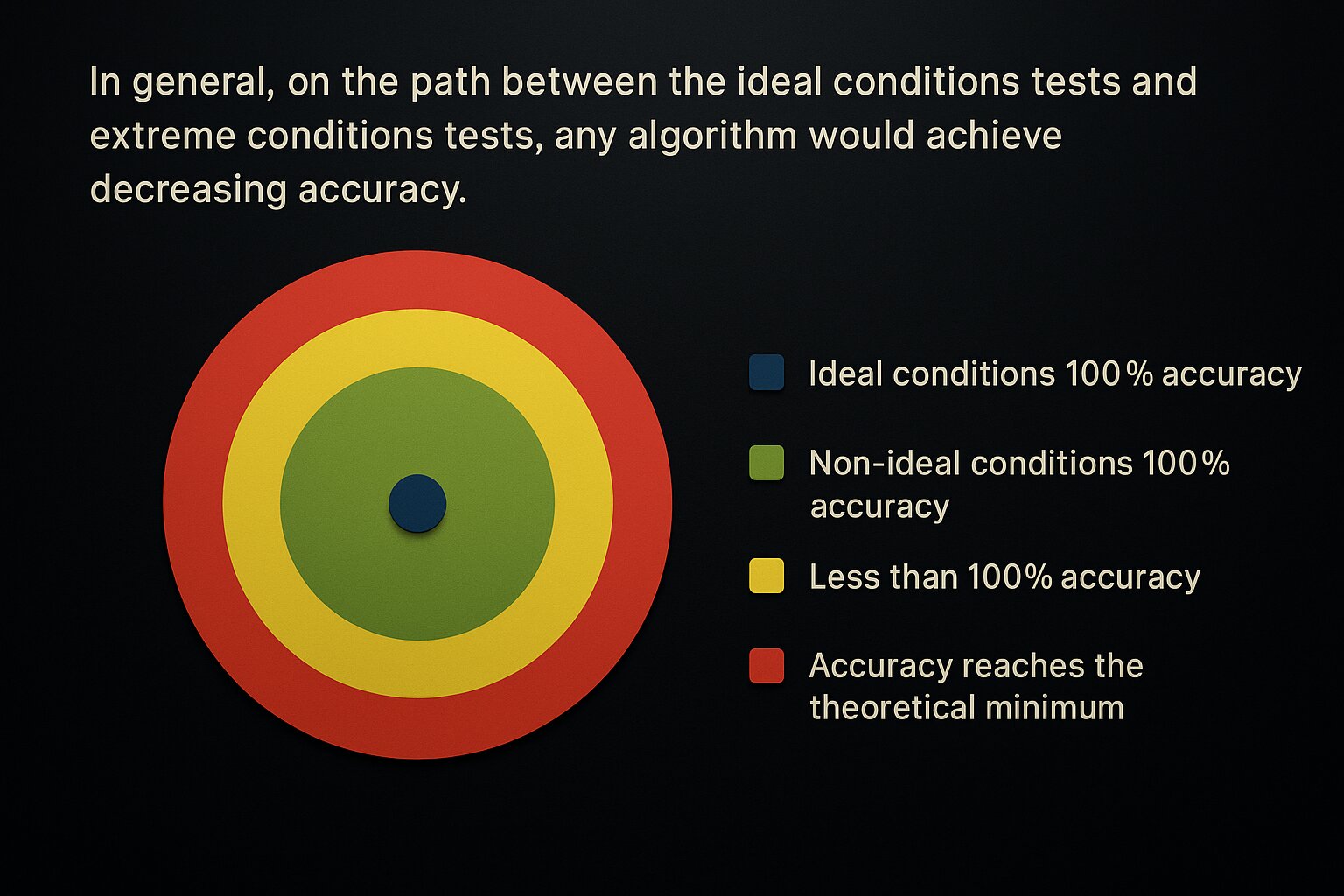
In ideal conditions, any simple algorithm can achieve 100% accuracy on certain tasks, such as computer vision. On the other hand, for any algorithm, regardless of its sophistication, there are extreme conditions in which its accuracy would reach a theoretical minimum. For instance, identifying an object from a test image that is perfectly identical to the registration image is trivial. On the other hand, identifying an object from a test image in which the object is 100% occluded is theoretically impossible and does not even make sense.
How do you even test such an algorithm ?
Since we could not use a widely recognized public test dataset to benchmark the algorithm’s accuracy simply because no such dataset exists for our specific problem, the accuracy figure alone may not be very informative. Accuracy is highly dependent on the test dataset used, which is a general fact. Therefore, to ensure meaningful and comprehensive testing, we made the following decisions:
(1) Test subjects:
|
We chose microchips as our test subjects because their surface features captured by camera are highly unstable with respect to the different scanning conditions compared to other products. This variability is primarily due to their fine structural details, surface bumps and reflectivity, which are sensitive to changes in scanning environments. In other words, they are some of the most challenging products we encountered in our physical tests. This choice gives confidence that the accuracy will not decrease when performing volume tests on other products. |
(2) Perturbation space:
|
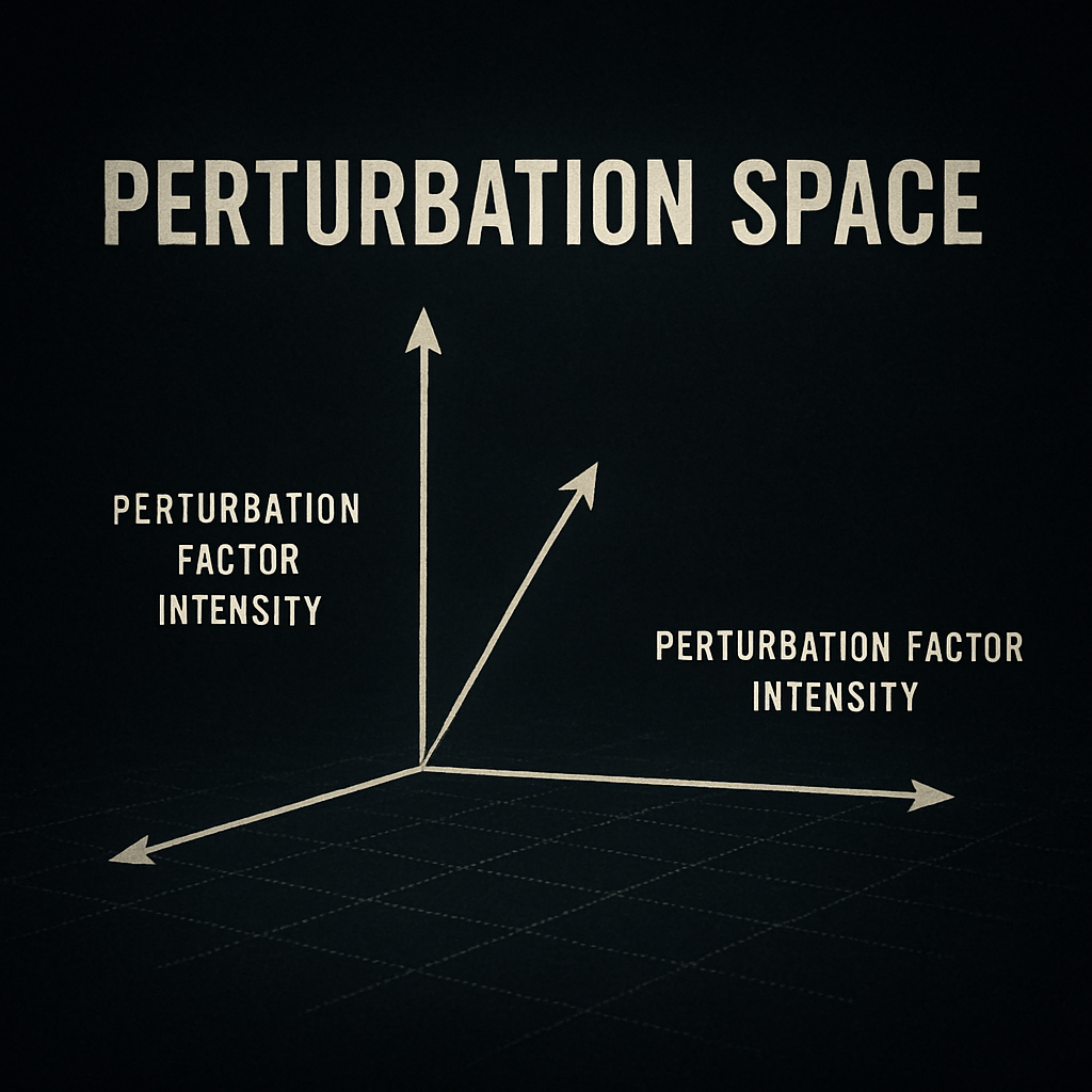
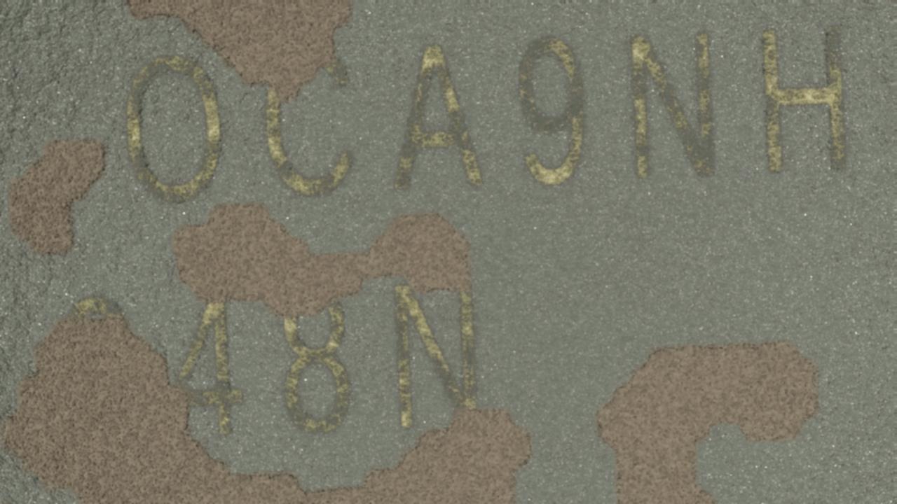
We decided to simulate random variations in conditions using different perturbation factors, such as misalignment, lighting, and damage. We refer to a combination of these perturbation factors as a perturbation vector, and the set of all possible perturbation vectors as the perturbation space. Our goal was to identify the largest simply connected region (i.e. with no holes) within this perturbation space where the algorithm consistently achieves 100% accuracy. Additionally, we aimed to evaluate how quickly the accuracy declines outside this region and to analyze how each perturbation factor impacts accuracy when studied individually across its full range of magnitudes. This approach was also chosen to validate that Amprenta algorithm accuracy is solely dependent on the magnitude of perturbations, rather than the specific test subjects. Our objective was to achieve definitive 100% accuracy, rather than an asymptotic approach to 100%, which would suggest gaps in the region of identifiable instances regardless of the extent of variations. |
(3) Fingerprints:
|
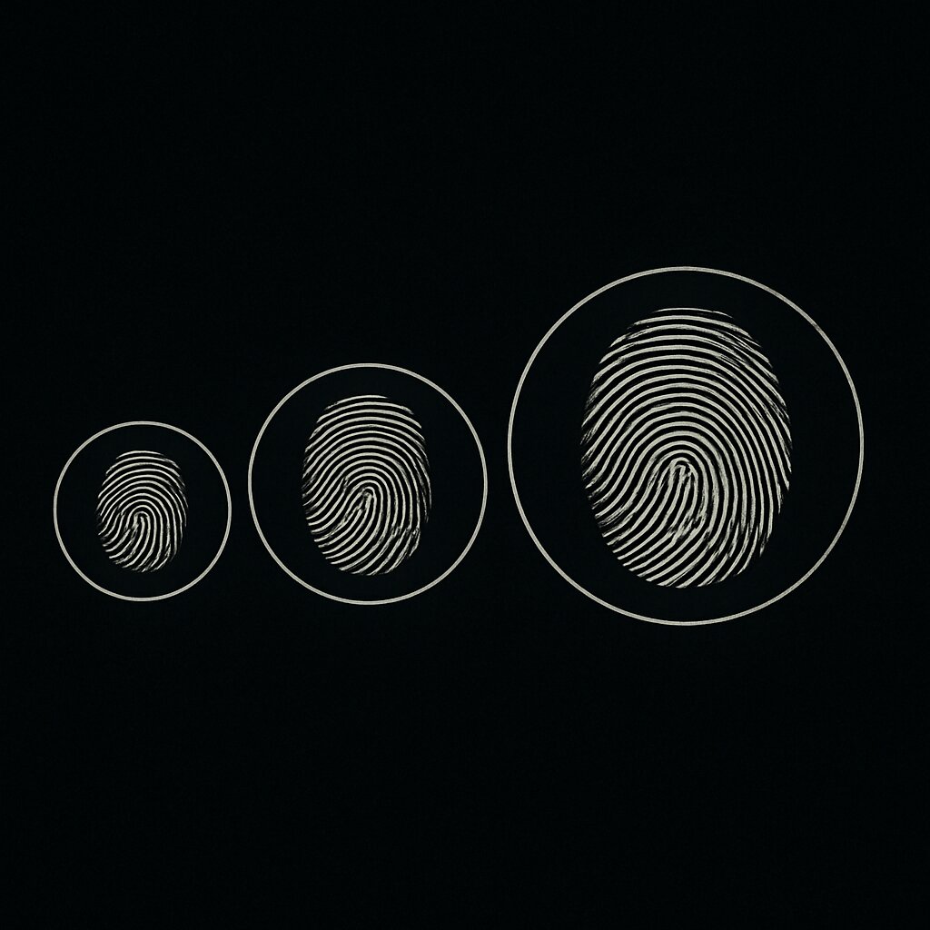
The algorithm’s identification power depends on the size of the fingerprint, a parameter adjustable by the user. A larger fingerprint increases identification power (i.e. accuracy) but decreases processing speed. This creates a trade-off between Fast Mode (smaller fingerprints, standard identification power, faster processing) and Deep Mode (larger fingerprints, higher identification power, slower processing). For our volume testing, we chose a smaller fingerprint size, corresponding to Fast Mode. By testing the algorithm under one of the most restrictive settings (Fast Mode), we ensure there is room to preserve high accuracy in more extreme scenarios by increasing the fingerprint size if needed. |
In summary, because we cannot predict the exact operational conditions required by different industry use cases:
- we chose the most challenging products we encountered;
- we ensured 100% accuracy across a sufficiently large and continuous range of perturbations;
- we opted for a small fingerprint size to allow for flexibility and potential improvement in accuracy under more extreme conditions.
An accuracy number alone is not enough !
An important theoretical consideration related to accuracy involves the topology of the no-errors region. There is a fundamental difference between a no-errors region that is simply connected (i.e. without holes) and one that is not simply connected (i.e. with holes).
To illustrate the practical impact of the difference between the two cases, consider the task of recognizing a symbol on a piece of paper in images captured from varying distances.
Suppose both Algorithm A and Algorithm B achieve a 90% accuracy on the same test set. However, examining their correct and incorrect answers relative to the distance from which the image was taken reveals distinct distributions of errors:
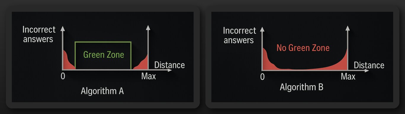
Algorithm A exhibits a “green zone”—an interval of distances where its accuracy reaches 100%. This implies that under practical and permissive conditions for image capture, Algorithm A can achieve perfect accuracy. In contrast, Algorithm B lacks such a zone, consistently producing some errors regardless of the conditions.
Similarly to Algorithm A from our example, the region in the perturbation space on which Amprenta algorithm achieved 100% accuracy is simply connected and has clear boundaries. This means we didn’t exclude any potentially difficult cases from our testing range. The conditions were rigorously defined, and within this range, every instance was accurately identified.
How was Amprenta accuracy measured ?
After we fixed a maximum intensity of each perturbation factor that is larger than any intensity encountered in our physical experiments in reasonable conditions, we generated random perturbation vectors in the perturbation space to obtain a large test data set.
Our test data set is accompanied by manifest files that contain the perturbation vectors applied to each synthetic microchip image.
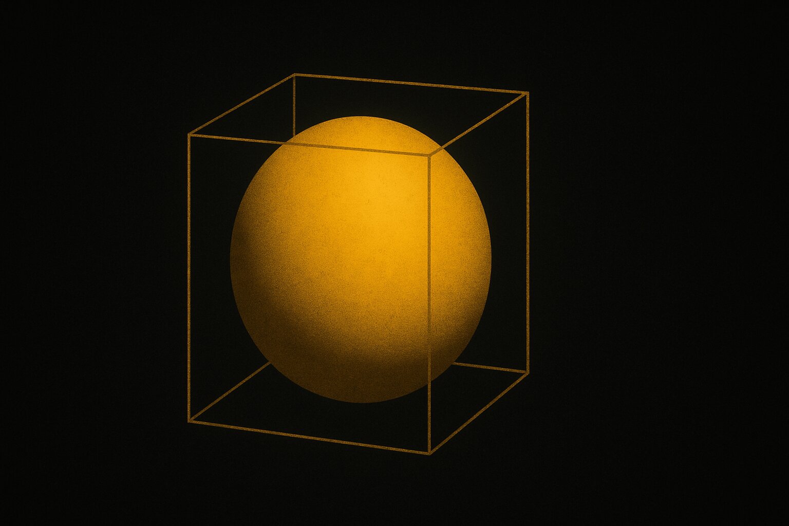
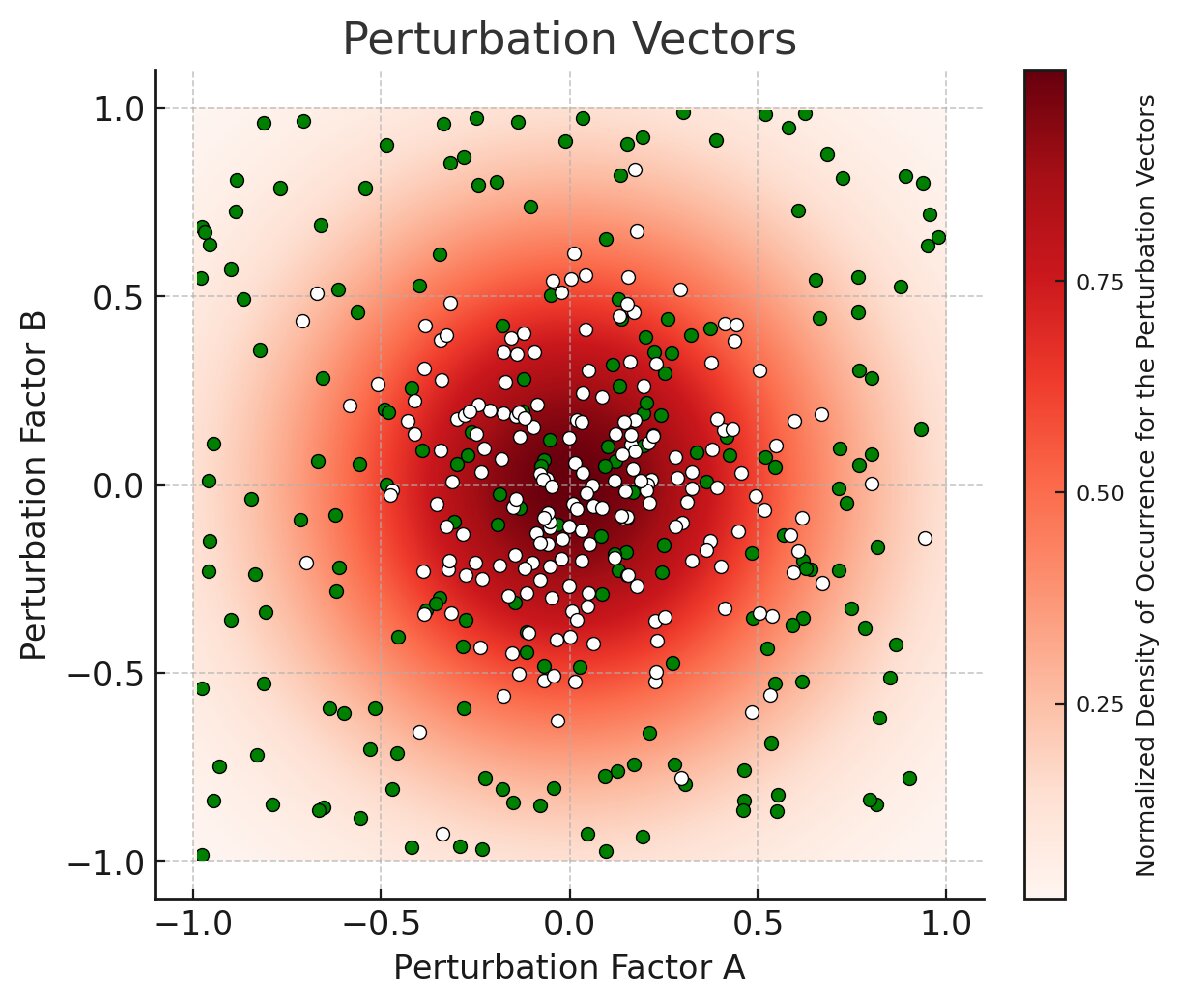
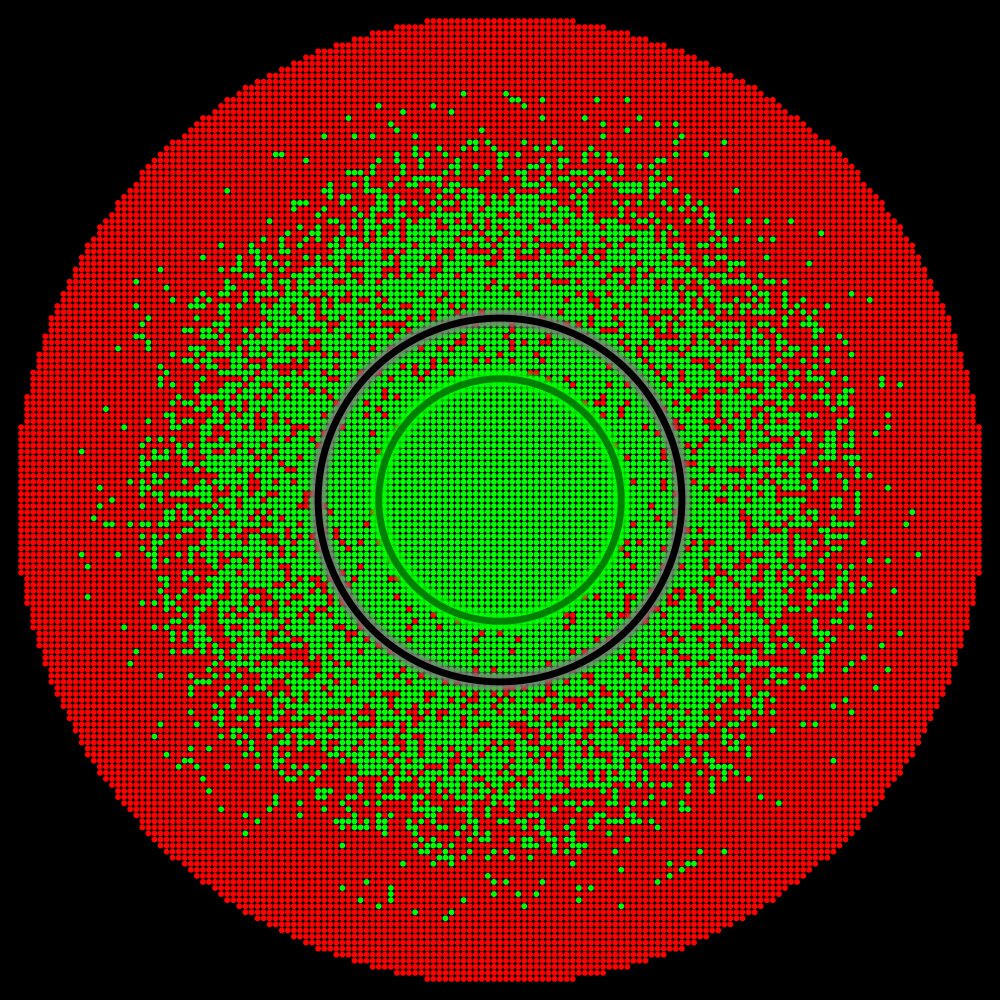
In reasonable operational conditions, natural perturbation vectors (orange dots) are typically expected to be randomly Gaussian distributed inside a hypersphere (modulo normalization), with the most extreme conditions corresponding to its boundary.
In our generated data set, artificial perturbation vectors (green dots) are randomly uniformly distributed inside a hypercube (modulo normalization), with the most extreme conditions corresponding to its corners.
Because the generated perturbation vectors are uniformly distributed, the test set remains balanced (i.e. gives a fair mix of all cases), which is crucial for correctly evaluating accuracy.
Moreover, the “curse of dimensionality” works in our favor. In higher dimensions, the bounding hypercube of that hypersphere has a much larger volume than the hypersphere itself. For instance, in 11 dimensions (the dimension of our perturbation space), the volume of the 11-dimensional hypercube is approximately 1087 times larger than the volume of the 11-dimensional hypersphere it bounds. In short, the green dots (representing perturbation vectors in our testing) cover a much larger space than the white dots (representing perturbation vectors expected in real-world applications).
Amprenta algorithm achieved 100% accuracy on the test data set. The result showed that our algorithm has a green zone that is more than large enough to include all the perturbations we encountered in the physical experiments. Outside this green zone, accuracy decreases very gradually (but false positives remain zero), meaning some instances may not be identified.
In other words, there is a ‘continuous’ region (the green zone) in the space of perturbation vectors in a (large) neighborhood 0 (0 representing the theoretical ideal conditions) where our algorithm achieved 100% accuracy.
|
From our physical experiments, we concluded that this region is large enough to encompass the perturbation vectors expected in real environments. To illustrate the decline in the identification rate outside the green zone: when we significantly broaden the range of variation for the perturbation factors, only approximately 1 to 3 instances out of a million will go unidentified. It’s also worth noting that even in the potential situation that the perturbation vectors fall outside of the green zone, the algorithm will not misidentify items. In the worst-case scenario, it will classify them as “unidentified,” thereby avoiding any false positives. This allows users to improve the scanning conditions and try again to obtain a match, if any. |
For example, this is the manifest for the 100% accuracy volume test #3 which defines the green domain:
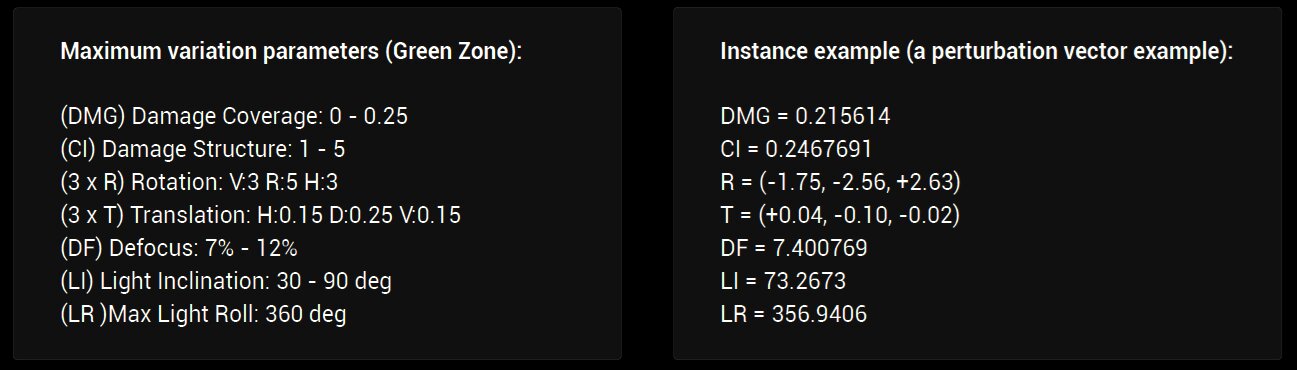
- We also applied softer perturbations to the registration images.
- We have significantly improved the robustness since then (i.e. increased the Green Zone size).
- Test size: 1 Million registered synthetic microchips + 10 Millions test images i.e. 10 images for each microchip in different conditions: different lightning, different focus, different alignment, different damage
Why does it make sense to measure accuracy using this methodology ?
The theoretical space of perturbation vectors is huge and a significant part of this space consists in perturbation vectors that either makes the identification theoretically impossible or they define highly unlikely poor conditions. Measuring the accuracy over the entire theoretical space will be more a characterization of the space structure itself from this point of view rather than a characterization of the algorithm power.
As an analogy, imagine trying to test how good a car is by driving it across every type of terrain on Earth — deserts, jungles, mountains, and even oceans. Instead of learning how well the car performs, you’d just end up discovering where there are roads. That’s because the car is designed for roads, not for every possible surface.
The same principle applies when evaluating a system or technology: if you test it across all imaginable scenarios instead of the relevant, intended ones, you're not really measuring how good the system is — you're just mapping out where it happens to work. To properly assess performance, testing must reflect the context the system was built for.
By analyzing the distribution of perturbation vectors during our physical tests, we estimated the extent of the perturbation space that likely corresponds to practical scenarios (illustrated by the interior of the black circle). The accuracy level within the interior of the black circle is crucial.
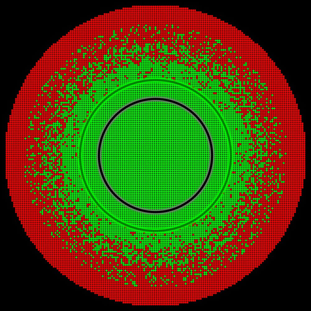
Situation A |
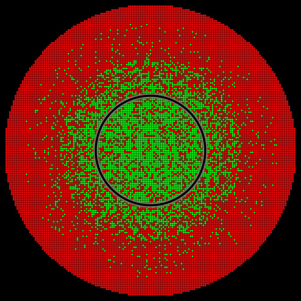
Situation B |
Situation C |
For instance, in “Situation B” where there is no green zone or in “Situation C” where the green zone is insufficient to cover practical scenarios the reported accuracy would have been less than 100%.
Amprenta exemplifies “Situation A”. Here, not only does the green zone completely cover the practical scenario region, but it also extends well beyond it, indicating robust performance across a broad range of conditions. In this situation, it makes perfect sense to report 100% accuracy.
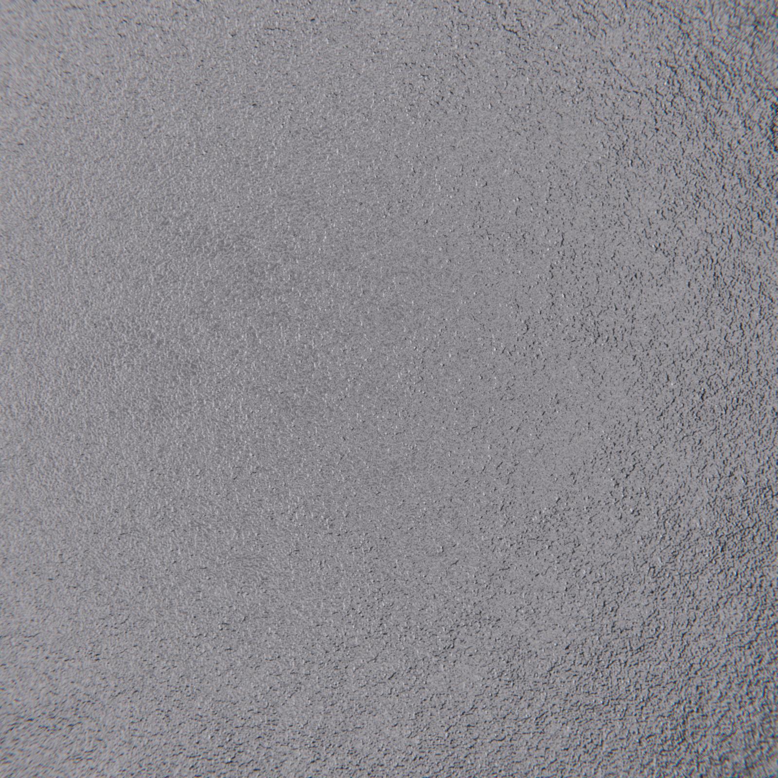
Typical examples from one of the 100% accuracy volume tests:
(1 Million Registered Images + 10 Million Test Images)
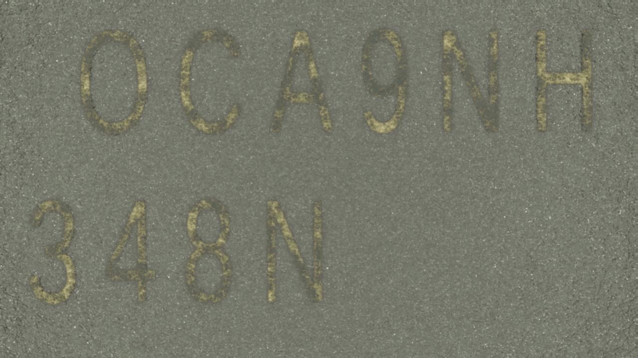
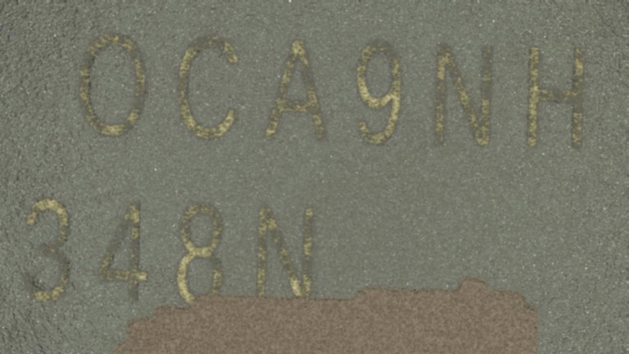
Microchip 1
Registration Image
Microchip 1
Test Image
Correctly Identified
Microchip 2
Registration Image
Microchip 2
Test Image
Correctly Identified
Microchip 3
Registration Image
Microchip 3
Test Image
Correctly Identified
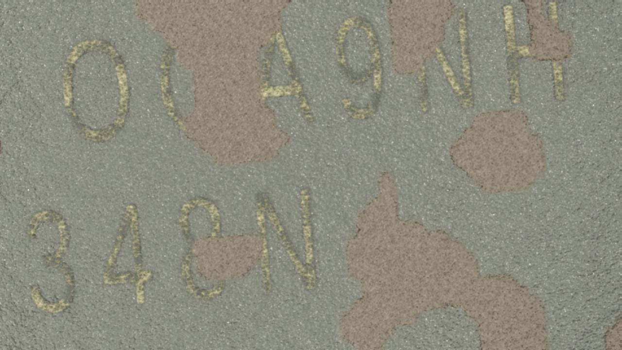
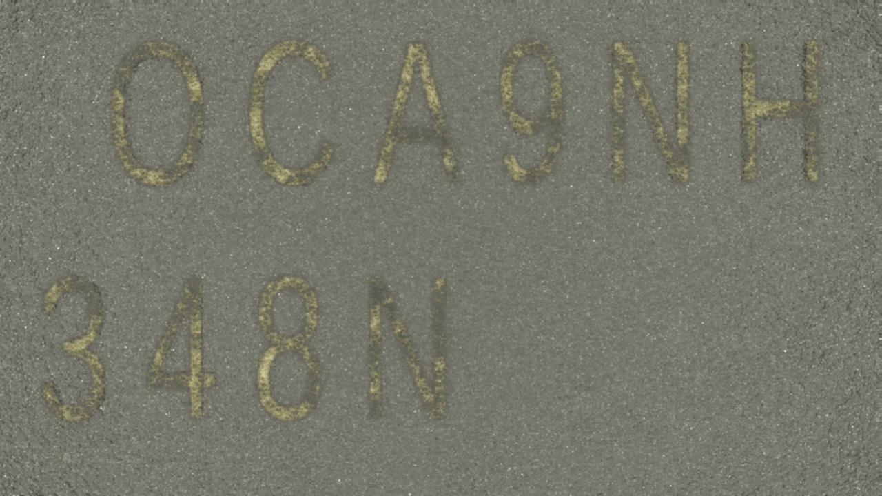
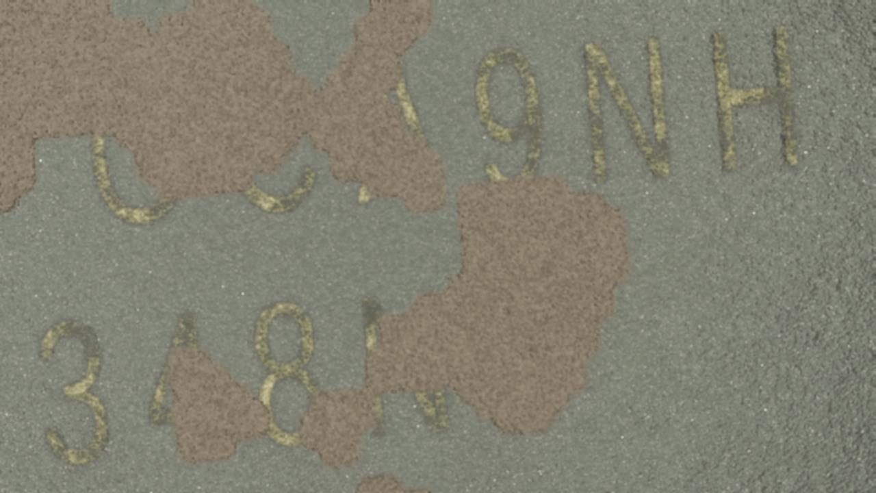
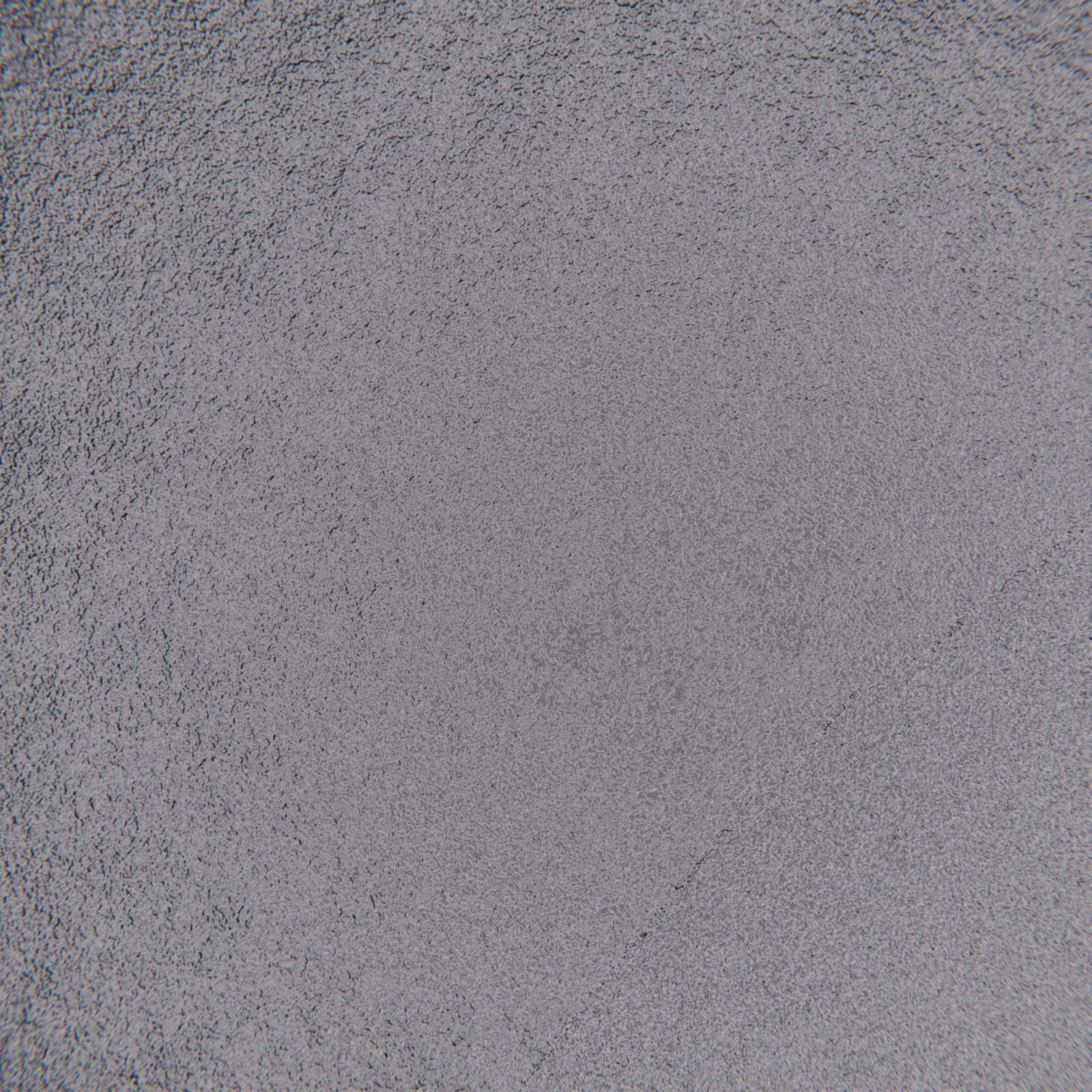
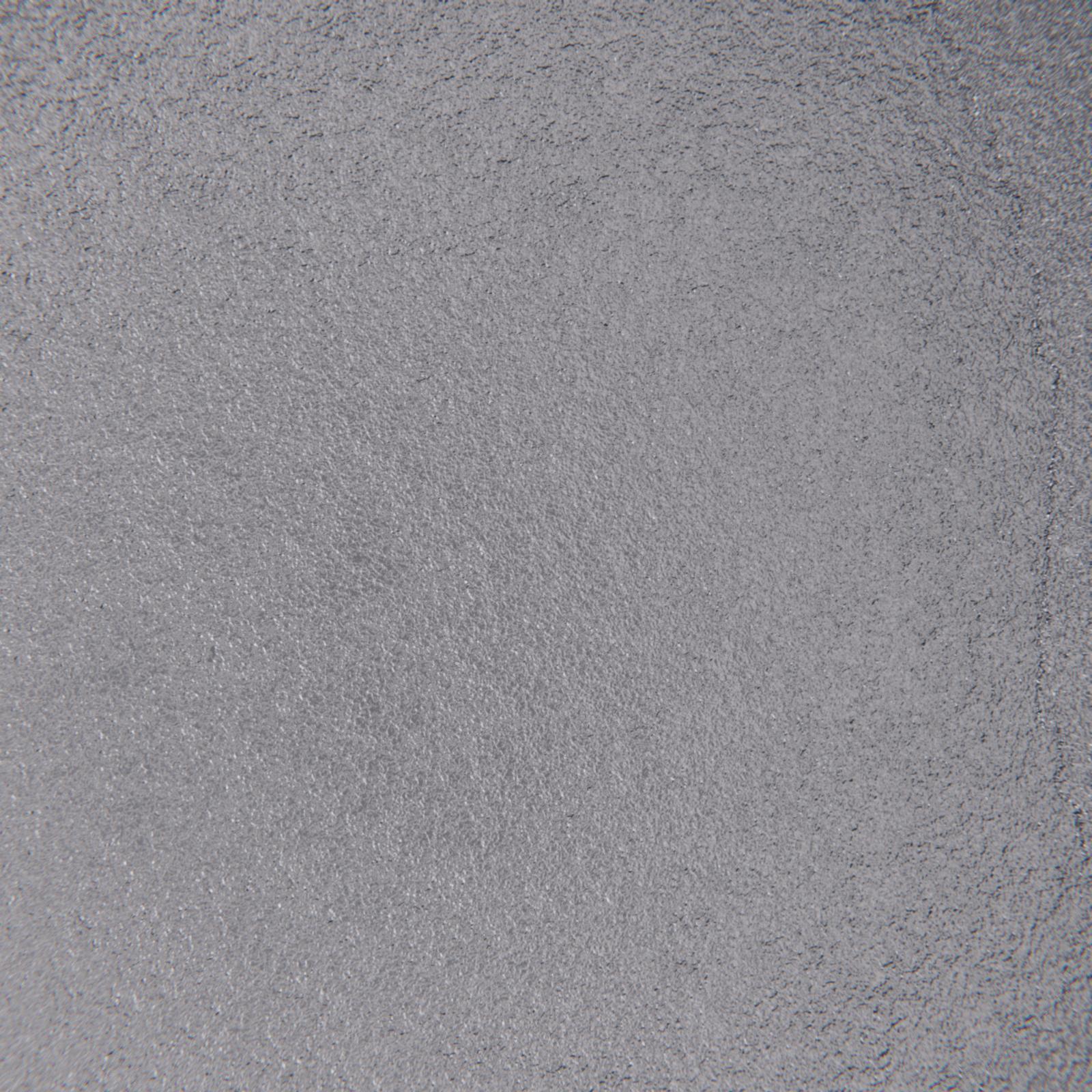
Testing the limits. Examples #1:
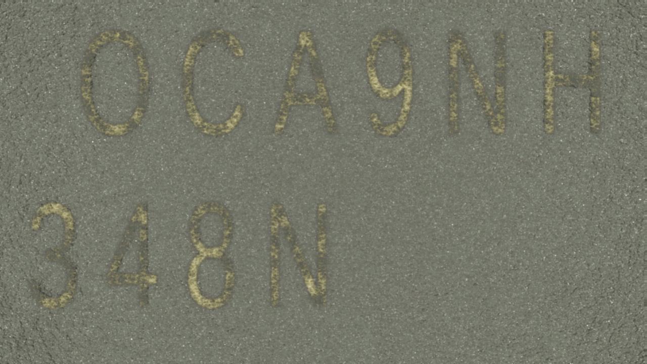
Registration Image
Test Image
Correctly Identified
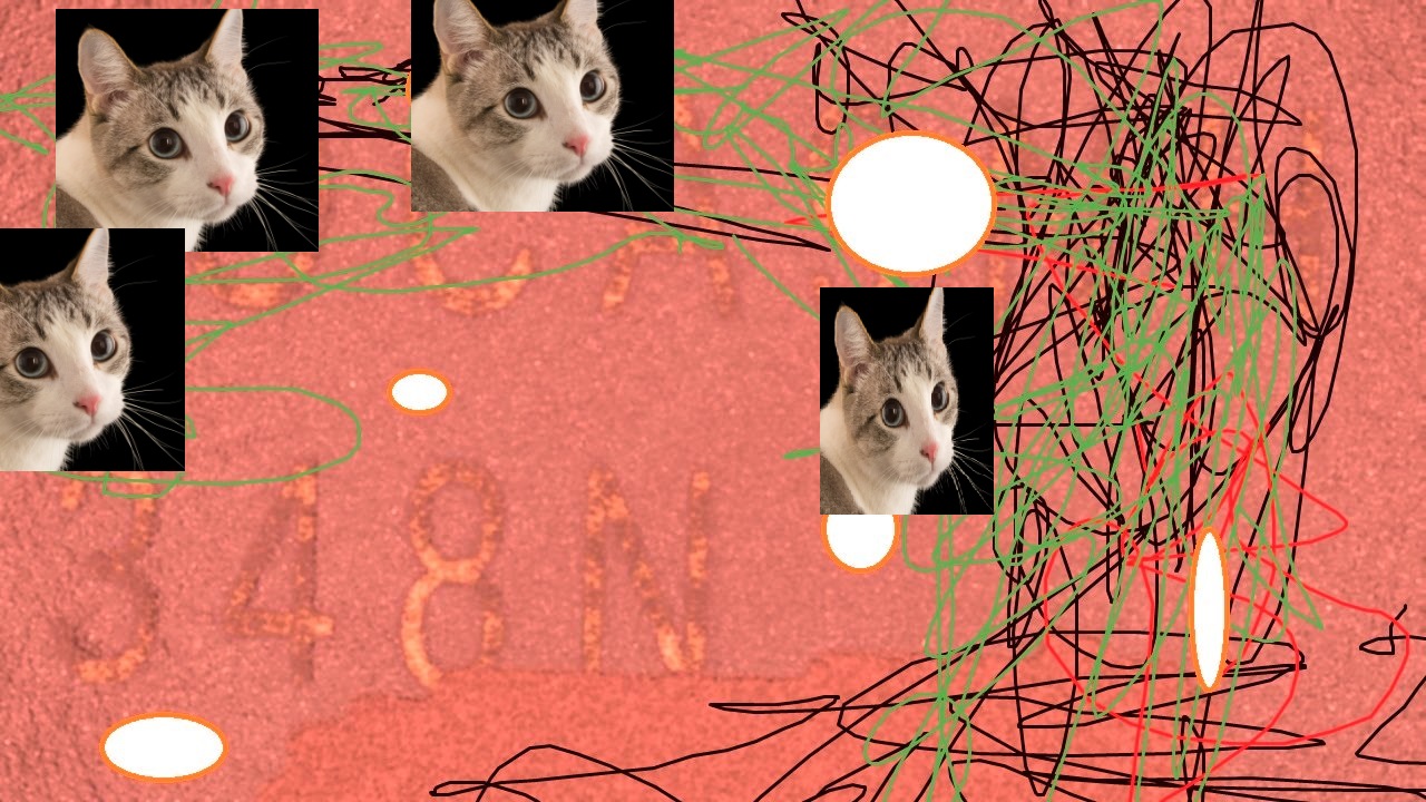
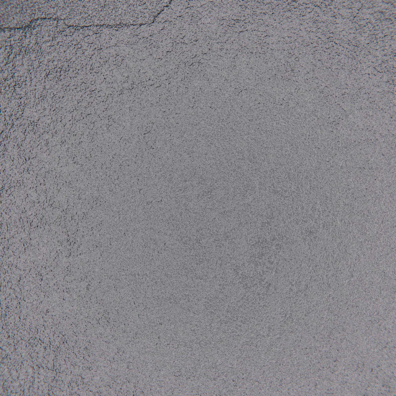
Test Image
Correctly Identified
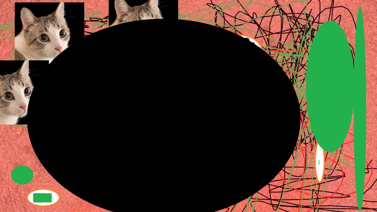
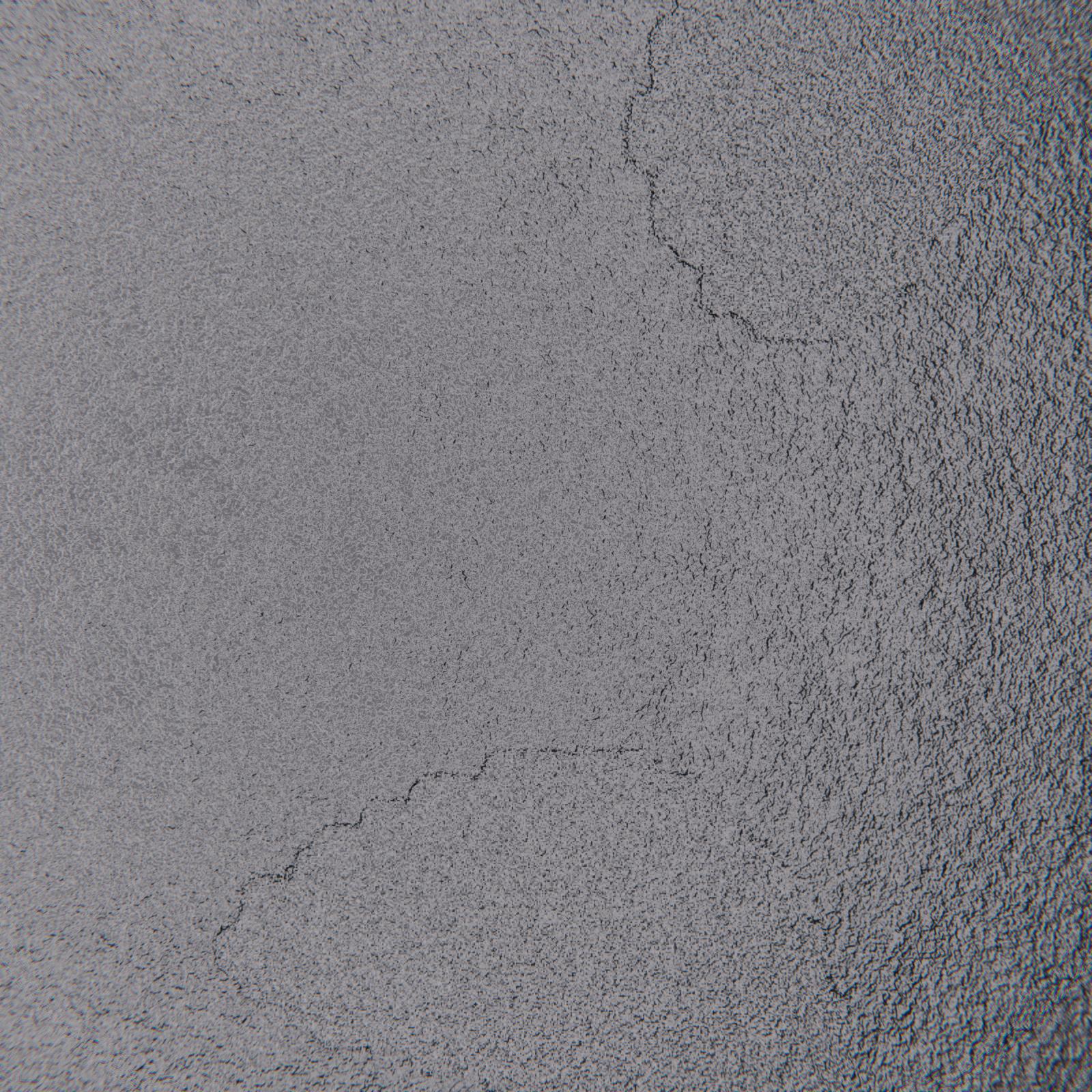
Test Image
Unidentified
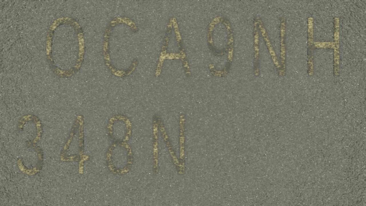
Testing the limits. Examples #2:
Surface A
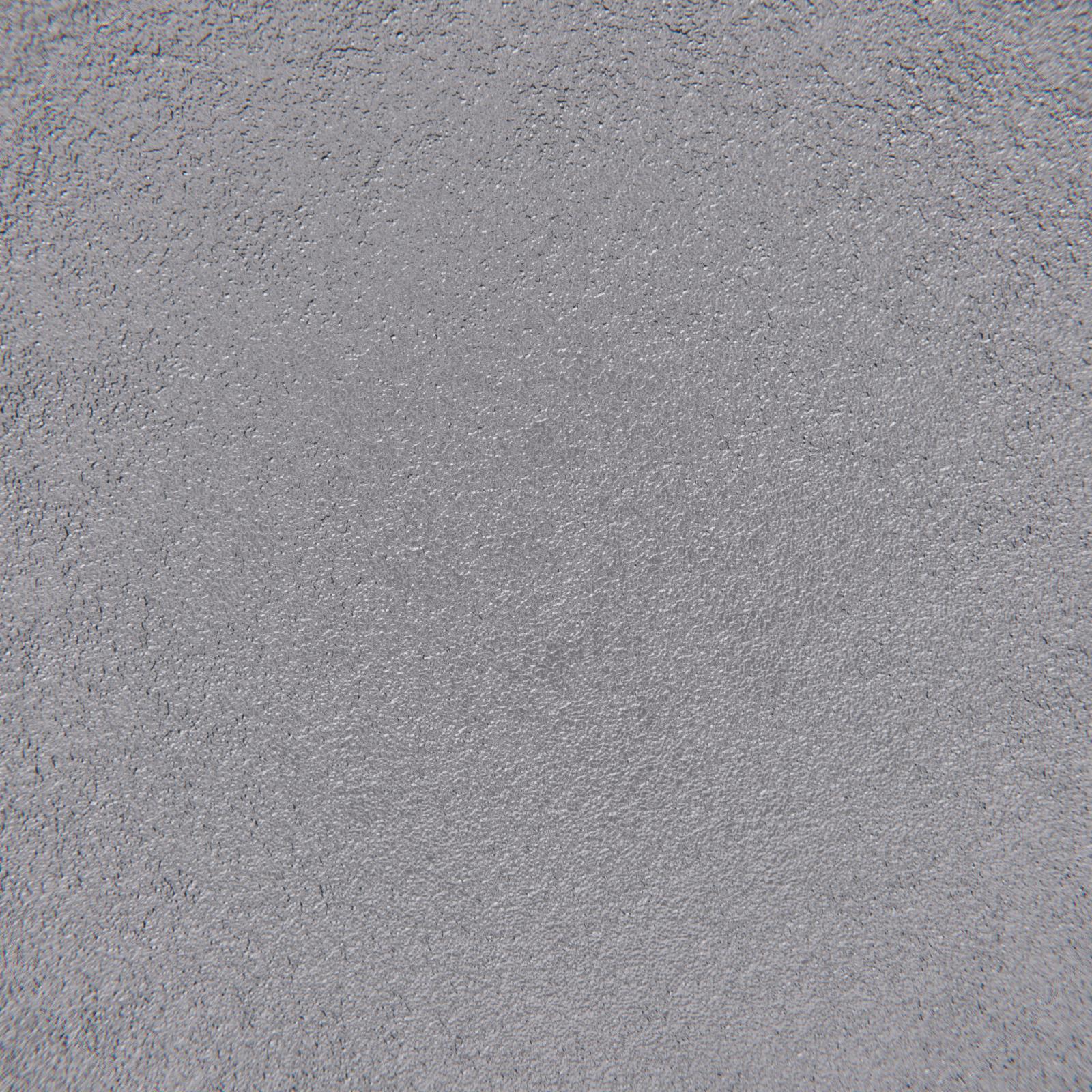
Registration Image
Test Image
Correctly Identified
Test Image
Correctly Identified
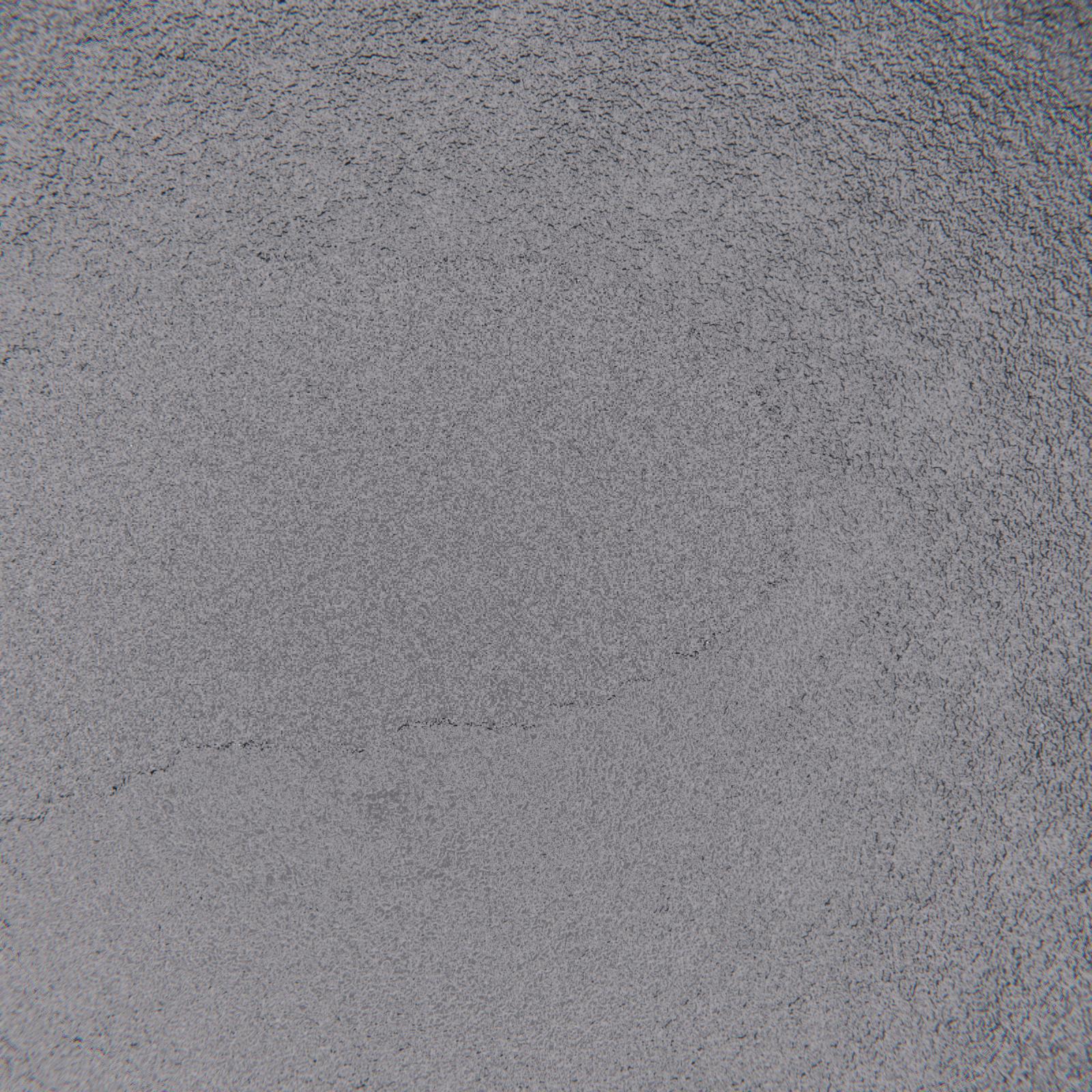
Test Image
Correctly Identified
Surface B
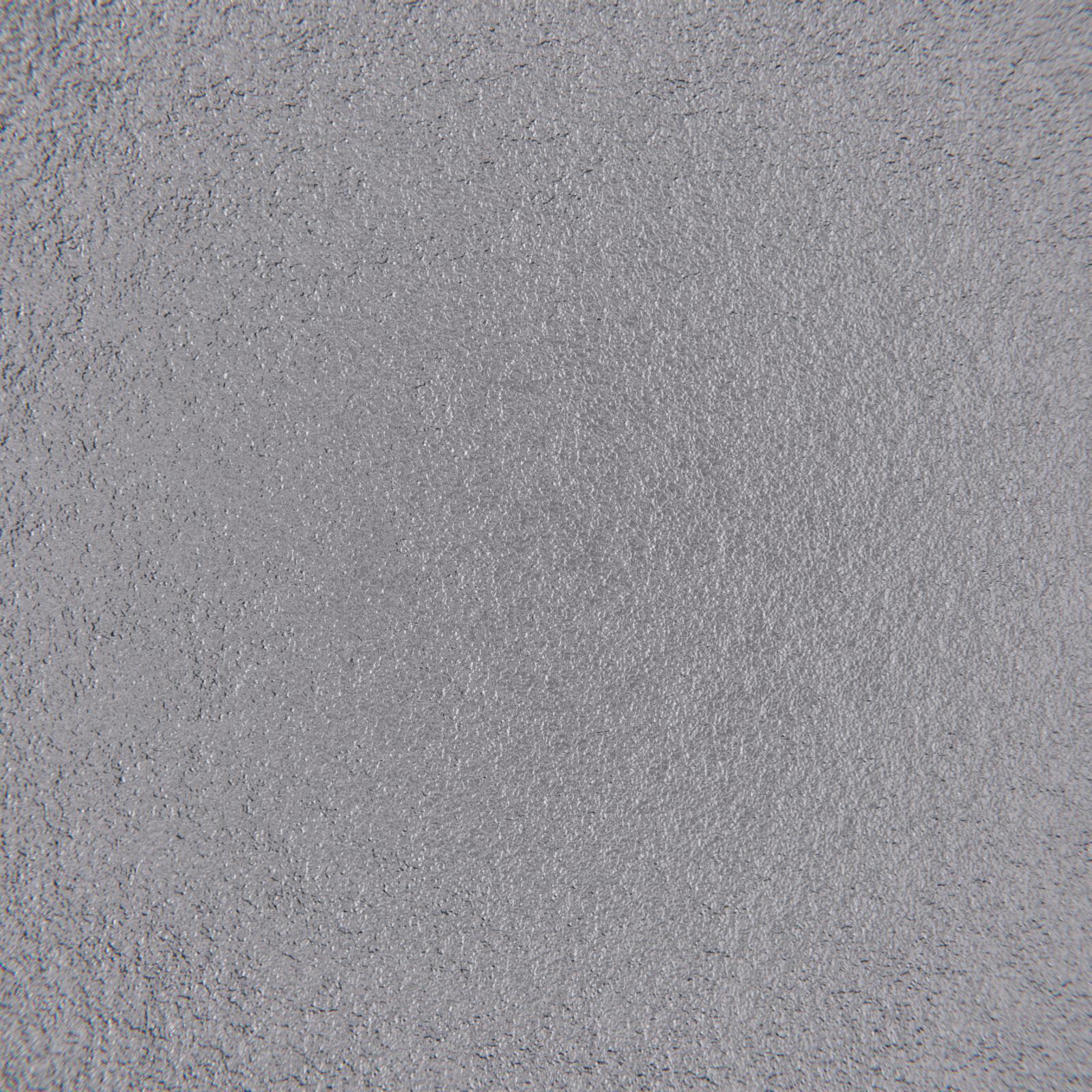
Registration Image
Test Image
Correctly Identified
Test Image
Correctly Identified
Test Image
Unidentified